It’s been a fair bit of time since my first attempt at simulating the ocean through a sum of sines approach. Now, I’m ready to tackle a more daunting, but much more appealing approach using the Fourier transform!

Where We Left Off

This blog post has been quite some time in the making, and it is the third post relevant to our journey to simulate ocean water. The first post discusses the process of transforming a flat plane into a surface that vaguely resembles water by adding waves of various directions, frequencies, and amplitudes together to offset its vertices. The second post discusses the Fourier transform, and is an intuitive introduction to the method we will use to enhance our ocean!

Right now, our understanding of the Fourier transform is that it is a formula to convert between a signal’s time domain and its frequency domain (also known as its spectrum). We can also take the inverse transform to add back together all of the waves. For our ocean simulation we can define a spectrum that is obtained from real oceanographic data, and use the inverse transform to generate a surface height map.

However, let’s take a moment to consider how this is different from what we did before. Both approaches sum together a variety of waves, but the spectrum for the sum of sines was generated using fractal brownian motion. So why do we need the Fourier transform? The answer lies in the time complexity of the algorithm.

Consider that as the size of our ocean grows (to be convincing, it needs to), the shader must add up waves for every point displaced. If the ocean is $n$ x $n$ vertices, the number of calculations is proportional to $n^2$. Therefore, we consider the algorithm $O(n^2)$, pronounced order $n^2$. As we scale our ocean, the number of computations grows too quickly to be reasonable. Here’s where the Fourier transform comes in: Using symmetry revealed by waves in the complex plane, the Fourier transform’s time complexity can be reduced! What a mouthful!

Unlocking the Fast Fourier Transform

Let’s explore how our sum of waves can be optimized. The first thing to note is that the formula for the DFT and IDFT are so close, and any optimization we make to one can be made to the other. Still, at an initial glance, both have a time complexity of $O(n^2)$. So how can we exploit symmetry? It’s not very intuitive to visualize, since there are so many different waves being added together. We’ll turn to the formula for the IDFT, since this is what our code will need to do. Remember that $x(n)$ is a sample of the time-domain at time $n$, $X(k)$ is the amplitude of the wave with frequency $k$, and $N$ is the number of samples in our signal:

We know that the Fourier transform is periodic over $N$ samples in the time-domain by definition. This means that if we add $N$ to the time, the expression should have the same value. Let’s build off of this idea. We can look a half period ahead, and see where this leads us. With a little help from the properties of exponents, as well as Euler’s formula, the new expression is pleasantly familiar.

The only difference between this and the initial expression for $x(n)$ is that the signs of some terms are flipped. More precisely, all of the odd terms are subtracted. But if we are clever, this doesn’t stop us from making an optimization. We’ll add all of our even terms together and store the sum, and do the same for our odd terms. To find $x(n)$, we add these two sums. To find $x(n + N/2)$, we take their difference. In practice, this is a nearly free way to save computing steps.

This is a great start. We’ve managed to cut the number of computations in half, and this really could significantly reduce our computation time. But this isn’t improving our time complexity. As we increase the number of frequencies, the number of calculations will still grow too fast, and crunching the numbers twice as fast just may not cut it. We need to keep the algorithm fast as scale grows, by keeping the number of computations low.

It’s not immediately clear how to do this, so let’s keep investigating our previous ideas and see where that leads us. We will take a closer look at the sums for our even terms, and then for our odd terms. Interestingly, it’s not very straightforward to separate our even terms and odd terms using the just equation we derived before. One method would be to list out some even terms, and derive a generic formula. The approach I prefer is to replace $k$ with $2k$, and cut the number of samples in half. This leads us to this equation:

Again, we remarkably get something eerily similar to the initial IDFT. There are two major differences. First off, we have half as many samples. However, the wave exponent doesn’t reflect this. Conveniently, both our numerator and denominator are twice as large as we’d like them. All we have to do is cut them both in half, and our problem is solved:

The only other difference is that we only sample the frequency of our even terms. This is actually pretty easy to get around, by placing the even terms next to each other, so that they can again be accessed with index $k$. What we are left with is a DFT! Let’s do the same thing for the odd terms. We can index them by simply adding one to the indices for all of the even terms. This one doesn’t play as gently, but we can break apart the exponent with some delicacy.

Thankfully, the term we factor out doesn’t depend on the frequency, so we only have to calculate it once. Then, once we solve the same problems as for the evens, we get another DFT! Here is our insight: The DFT can be calculated using two half-length DFTs and a small combination step!. Alone, this isn’t much, but we can recursively apply this rule. Therefore, a large DFT may be split into two medium DFTs, which are again divided into four small DFTs. This repeated divide-and-conquer algorithm is known as the fast Fourier transform (FFT). Our pseudo-code inverse FFT implementation may look something like this, and can be implemented using a recursive algorithm.

function IFFT(amplitudes)
{
  N = amplitudes.length

  // base case (amplitude = signal)
  if (N == 1) return amplitudes[0]

  // assert the number of samples is otherwise even
  assert(N % 2 == 0)

  // run the transform on the evens and the odds
  evens = IFFT(amplitudes.evens)
  odds = IFFT(ampltidues.odds)

  // combine the two transforms together to get our result
  for (n in [1,...,N/2])
  {
    // multiply odd factor by twiddle factor
    odds[n] *= eulers(2 * PI * n / N)

    // reuse the amplitudes array for our final values
    amplitudes[n] = evens[n] + odds[n]
    amplitudes[n + N/2] = evens[n] - odds[n]
  }

  return amplitudes
}

Wonderful! Again, there are so many ways to take this further. For now, we only support inputs with lengths of powers of two. This is okay, but there are versions of the FFT that support all sorts of lengths, and it’d be interesting to explore how these work. Another problem that we face is that our program is moderately optimized for computations, but it’s not optimized for memory usage. Each stage allocates (depending on implementation of the pseudo-code) two arrays, but it’s possible to use only a single array for the entire algorithm, cleverly swapping around values using a bit-reversal and butterfly network.

There is no shortage of rabbit holes to investigate, but a final one I’d like to investigate on is the time complexity of the FFT. We know that our DFT has turned into a repeated combinations of smaller DFTs. But how many times do we do this. Each time we combine, we double our DFT size. Therefore, we need to figure out how many times we double the smallest DFT (length-2) to get to our final size (length-n). This is equal to the base two logarithm of $n$. Each combination step requires that we pair up half our data with the other half, and so the amount of calculations is proportional to $n$. To get our total complexity, we multiply the number of combinations, by the number of instructions per combination to get $O(nlog(n))$. Let’s graph the approximate number of calculates for each type of complexity.

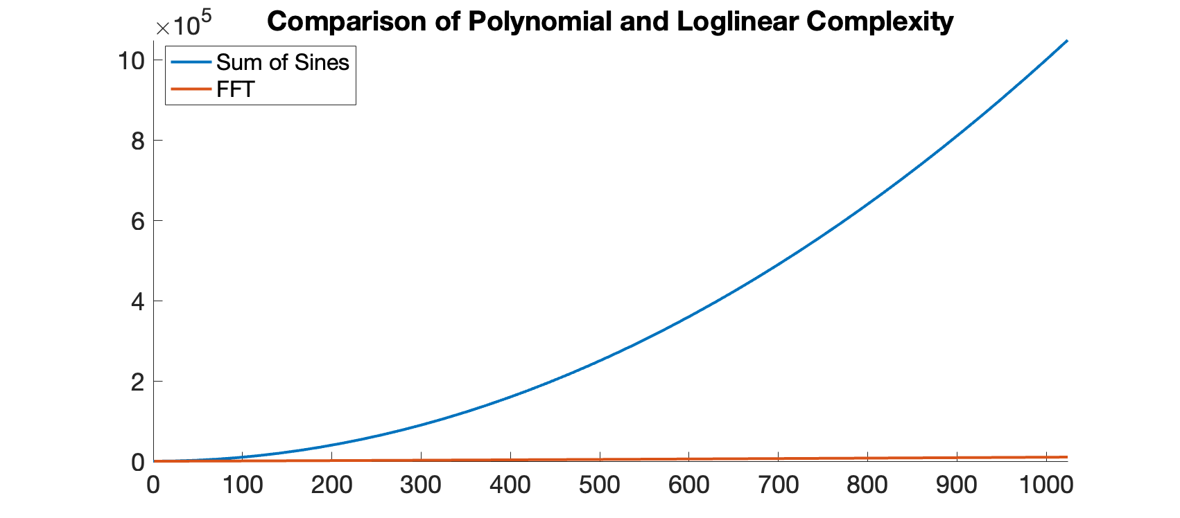
At small sizes, the two algorithm both use a small number of steps. but we can see a larger difference as we scale up. For an FFT with $1024$ samples (a reasonable size), the number of instructions for our new FFT-based approach is virtually nothing compared to the old approach.

Our Oceanographic Model

Trying to apply the Fourier transform to our ocean is tricky, but we can think of the height of the ocean as a 2D-signal through space. We haven’t dealt with more than one dimension before, but a two-dimensional signal simply repeats in two dimensions instead of one. To store our 2D-signal, we can use a texture, where each pixel in our texture represents a different point in the ocean, and it’s brightness represents the height.

We are used to using the Fourier transform (technically its inverse) to calculate a signal as it changes through time, but we are now using it to model a signal through space. Therefore, to avoid confusion, I’m going to from now on refer to the time-domain of our signal by its other name: the spatial-domain.

This system will be great! Let’s consider how we can prepare our spectrum so that we can use it to generate the ocean surface. Our new system must account for a new problem: a 2D-signal has a 2D-spectrum. It’s hard to understand exactly what this entails. Consider that with a 2D-spectrum, we have 2D-frequencies. Thankfully, the term 2D-frequencies is a sort of giveaway, because we understand that frequencies are two because they are just the frequencies for each direction. Take a look at the heightmap for a signal with an $x$-frequency of $2$ and a $y$-frequency of $3$.

Hopefully this makes things a little clearer. Now, we can choose a model for generating a spectrum. I chose to use the Jonswap spectrum, which is one model based on oceanographic data. It a uses the wind velocity and gravitational to approximate the intensity of waves of different frequencies. By combining the jonswap with some gaussian noise to model the probability of each frequency being present we can get a wide variety of possible oceans.

Let’s look at this spectrum and the heightmap that it generates. To interpret the spectrum, the pattern is that the frequency of a point is based on its distance from the center in the direction of the point and the amplitude is the brightnesss of the pixel. To visualize, we’re going to look at a simpler spectrum which culls points that aren’t in the same direction as the wind. It’s strongest waves are also lower frequency, which is similar to our fractal brownian motion from before.

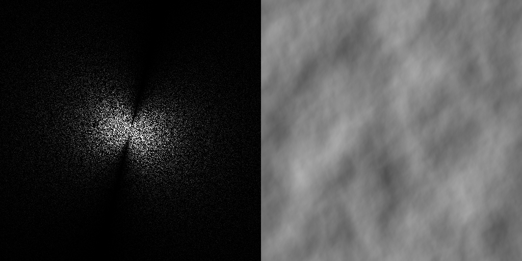
You can totally see the ocean surface in the texture! Now it’s a matter of implementing this into our simulation… It only took me three months. There are many reasons, but the biggest is that this project uses OpenGL, which doesn’t support compute shaders on macOS. It took some serious work to beef up the renderer to work with Apple’s own flavor of graphics, Metal.

We can effectively drop in the heightmap as a replacement for our old sum of sines vertex shader, sampling our texture instead of summing our waves. However, we run into a problem with our lighting model. Our diffuse lighting require surface normals, which we’ll need a new approach to generate. We can use a similar approach to before, calculating the binormal and tangent vector using the gradient. It’s interesting to take the derivative of the Fourier transform, but we end up with is another transform with a slightly modified spectrum. Therefore, normals are just two extra FFTs away.

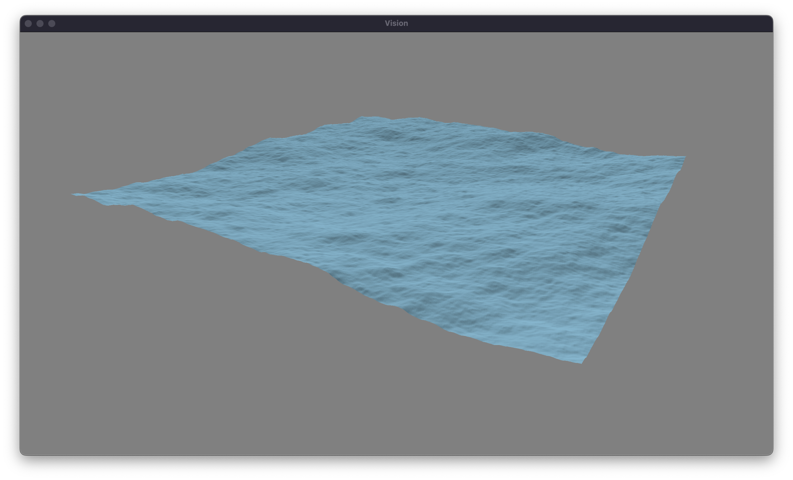
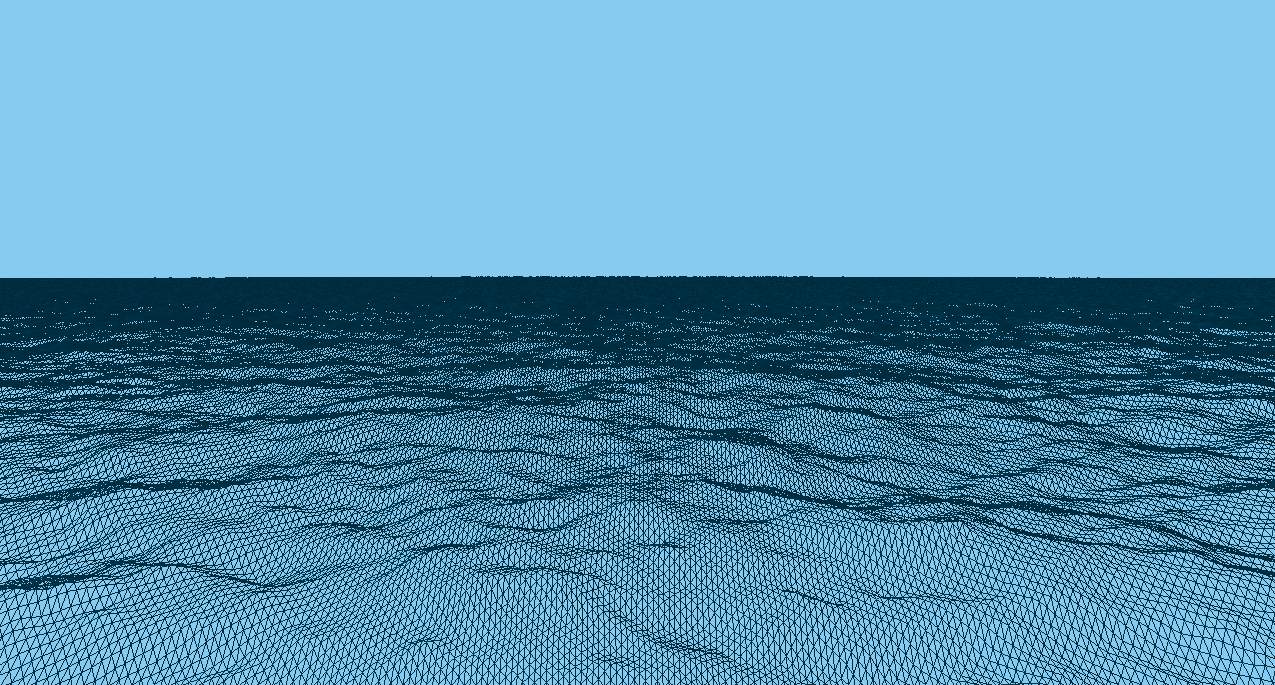
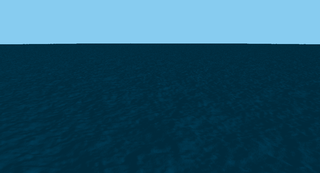
With all of these changes made, we have a new physically-based system for modeling the ocean! Here is a $25$ meter by $25$ meter plane rendered using our system, and our same old diffuse lighting.

Expanding Our Horizons

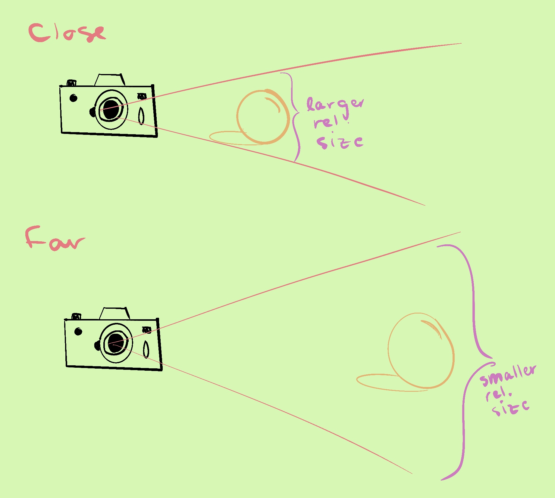
There are two big bottlenecks that we still need to resolve. First and foremost, our ocean is very small. We are only able to simulate a small patch. How can we possibly simulate a vast ocean while still retaining the visual fidelity that our simulation achieves? The trick is that we don’t have to. There are several approaches to this problem, but regardless the trick is to use perspective.

At further distances, the field of view of the camera covers a larger area, growing proportionally to the distance. This also means that detail becomes less noticeable. This insight can be used to determine that the projection of the camera scales the x and y coordinates of a point relative to the camera based on it’s depth.

If we want a crude way to preserve the x and z coordinates so that they maintain their uniform spacing after the transformation, we can multiply them by their depth from the camera. Let’s note that this is not perfect, because the x-z plane is not exactly perpendicular to the camera. However, when the plane is less perpendicular, it is viewed at more of a grazing angle, and the depth is less important. Let’s take a look at our new vertex shader.

void main()
{
  // Start with our plane centered about the origin.
  vec3 pos = a_Pos;

  // Compute the view direction and position of the camera.
  vec3 cameraDir = normalize(u_ViewInverse[2].xyz);
  vec3 cameraPos = u_ViewInverse[3].xyz;

  // To rougly prevent distortion, we multiply by the depth.
  vec3 toPlaneDir = pos - vec3(0.0, camera.y, 0.0);
  float depth = abs(dot(cameraDir, toPlaneDir));
  pos.xz *= depth;

  // Center the fine detail of the plane around the camera.
  pos.xz += cameraPos.xz;

  ... Shift our plane based on FFT data ...

  // Project into device space to render.
  gl_Position = u_ViewProjection * vec4(pos, 1.0);
}

Since some of the plane will have a negative depth, it doesn’t matter what we do with these points (as long as they don’t end up in camera’s view). One solution is to multiply vertices by the absolute value of the depth, so the vertices with negative depth don’t get flipped around in front of the camera.

Now, we have our ocean, but how do we fill it in with data? One option is to simply let the ocean repeat. Due to the periodic nature of the FFT, we can tile our pattern. However, we have another option. We can run multiple simulations. The FFT is so efficient that it is low cost enough to have multiple simulations running. We can have one that has all of our small waves, another with medium waves, and a final with our largest waves. This way, we don’t get repeating waves for a large distance, and we still maintain the high detail. The only thing to note, is that we need to restrict each wavelength to only one simulation, so that we don’t double count. Let’s implement this, and take a look at how this affects our ocean.

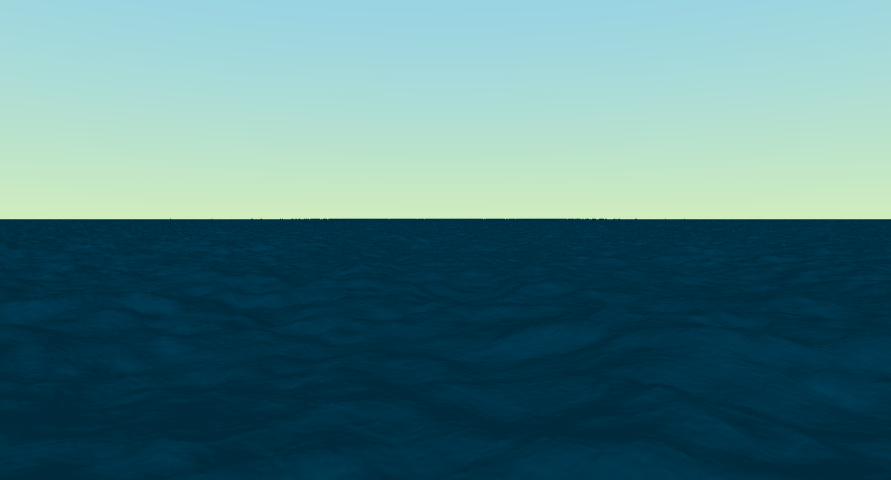
Now, we have a simulation where we cannot see tiling. Since each simluation is a diffierent size, we can maintain the detailed waves without having to see the periodic nature of the smaller FFTs!

Setting the Scene

There is still so much that we could do to improve the ocean, but I want to end this post by adding a few finishing touches. First off, I want to add a skybox to give our ocean an environment to live in. To do this, we will draw a cube mesh around the origin. Then, when we render it, we will strip the camera’s translation componenent. This will give us the apperance that we are inside a box that doesn’t moves. Let’s write some code to test this out, and see how it looks. Here is our vertex shader.

void main()
{
  // Reset the translation component of the camera.
  mat4 cameraMatrix = u_ViewProjection;
  cameraMatrix[3] = vec3(0.0, 0.0, 0.0, 1.0);

  // Project using the new matrix.
  gl_Position = cameraMatrix * vec4(a_Pos, 1.0);
}

Now, we need to color this box. We can use the position of the box in space to do this. We can treat the coordinates as an arrow, and use them to sample a cubemap texture, or define our own function in the fragment shader. For now, I’m going to write a function that uses the height of the position to define a color gradient.

vec4 SampleSkybox(vec3 direction)
{
  // Normalize the vector to get a unit length.
  vec3 dir = normalize(direction);

  // Compute the height above horizon (horizon = 0)
  float height = dir.y;
  
  // Use the height to interpolate between our sky and horizon color.
  return mix(horizonColor, skyColor, height);
}

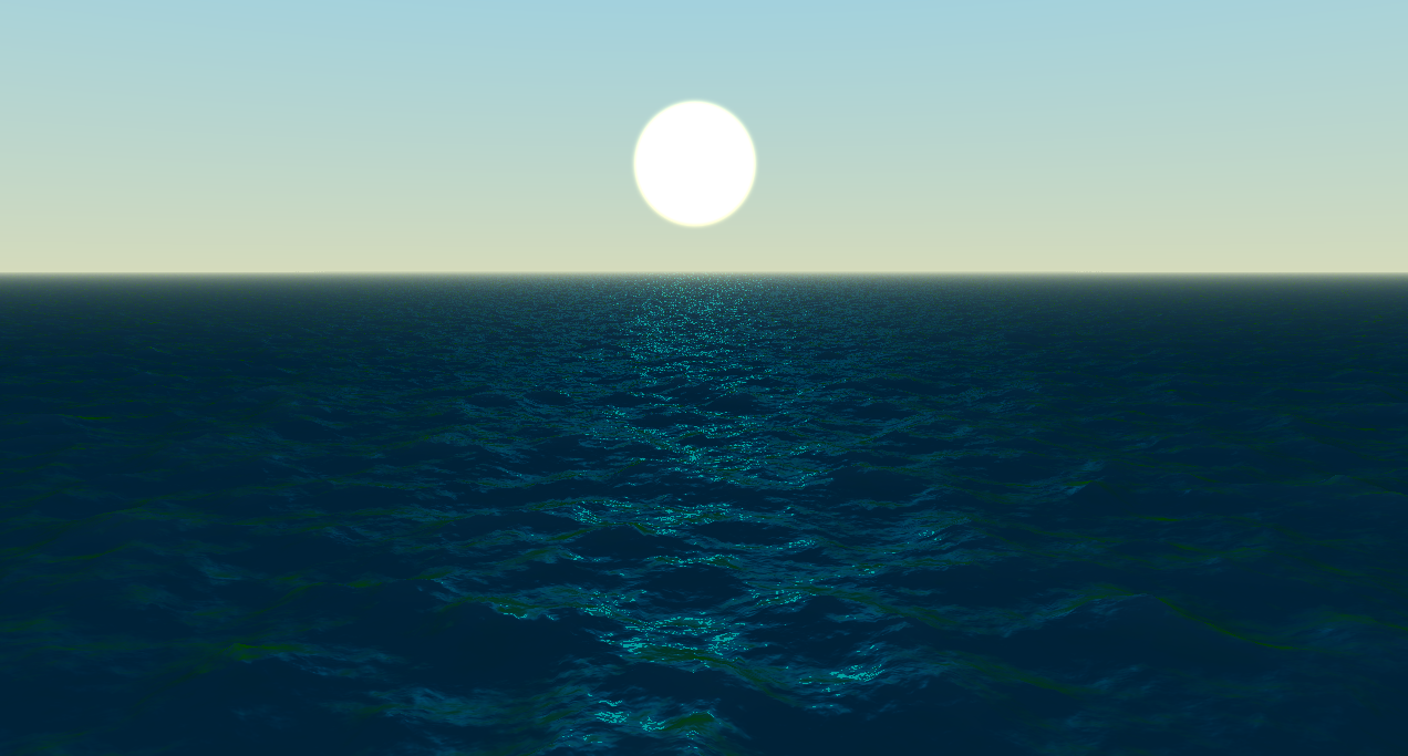
This looks decent, but we could really use a sun in our sky. Let’s choose some direction to be the direction of the sun, and find the angle between the sun and our direction in the sky using the dot product. If we do this, we can set a threshold to mix between the sky and the sun color. However, we want the sun to be white, so we can amplify the sun’s color in the mixing, as if we are overexposing it.

vec4 SampleSkybox(vec3 direction)
{
  // Normalize the vector to get a unit length.
  vec3 dir = normalize(direction);

  // Compute the height above horizon (horizon = 0)
  float height = dir.y;
  
  // Use the height to interpolate between our sky and horizon color.
  vec4 skyGradient = mix(horizonColor, skyColor, height);

  // Use a smoothstep to fade between the two colors.
  float sunCosine = dot(dir, sunDirection);
  float sunInfluence = smoothstep(sunThreshold - sunFade, sunThreshold, sunCosine);

  // Multiply the sun color by a factor of two to overexpose it.
  return (1.0 - sunInfluence) * skyGradient + (2.0 * sunInfluence) * sunColor;
}

For now, I’m going to leave the sky here. But I’m going to add a few finishing touches tie everything together. There are a lot of fancy lighting models that I’d love to explore in the future, but for now, we can approximate water shading by adding two factors to our lighting model. First, we can add specular reflections to the surface. While Lambert’s cosine law captures the magnitude of indirect light that reaches the camera, specular reflections capture light that bounces directly from the source to the light. This can get complicated quickly, but we can reflect the direction towards the camera around the normal of the surface and then compare that to the sun direction in a similar manner to before. Additionally, we estimate subsurface scattering by adding a term proportional to the height of the water. This is a pretty over-simplified model, but if we combine it with reflections by multiplying all of the terms by the color of the reflected skybox, we will have a pretty convincing ocean. Finally, we add a post processing based fog shader to blend the horizon with the skyline. I’m super happy with how the ocean ended up looking.

I may revisit this project in the future, as there is still so much that could be done, but I have a few other ideas that I’m hoping to explore. While I’ve really enjyoed this project, the scope was very large for a single blog post, so I unfortunately had to skip over a lot of the details and optimizations that made me enjoy this project the most. I think that I will keep this in mind as I move forward on these types of projects. Still, I learned so much about graphics programming, and I solidified that knowledge by putting theory into practice. You can check out the source code for this project here!

References

• GPU-Efficient FFT
• Empirical Directional Wave Spectra for Cpmputer Graphics