Discovering the Fourier Transform

In my adventures with fluid simulation, I came across something called the Fourier transform, a powerful algorithm used throughout many fields of science. Having no idea how it worked I took a step back. In this article, I will explain the realizations that have helped me understand the Fourier transform, and we’ll use it to create a drawing program!

Background

The Fourier transform is one of the most abundant algorithms in all of modern mathematics whether you realize it or not. So let’s define it: The Fourier transform takes a signal and breaks it into its frequencies. The inverse Fourier transform takes different frequency signals and recombines them.

Let’s just wrap our heads around what this means. One of the most common signals that we deal with is sound. What does it mean to break a sound wave down into its frequencies? Consider a piano chord, consisting of several different notes played together. By taking the Fourier transform of our piano chord, we convert it into the notes that break it up. From there, we can remove the notes that we don’t like, and then put them back together.

Here’s some vocabulary so we’re all on the same page. Our signal is going to have a value over time, so this is called the time-domain. In the case of our piano, this is the vibrations of air that makes you hear a chord. After we take the Fourier transform, we have the set of frequencies (notes) which made up the chord to begin with. This is the frequency-domain, which is also sometimes called the spectrum of frequencies.

In general, the genius of the Fourier transform is hidden in the complex situations where it is most useful. And while the underlying idea is simple, putting it into practice requires some fairly involved math. I will attempt to give the necessary background, but I’m going to assume comfort with single variable calculus. Calculus is an integral (no pun intended) part of the Fourier transform, but we’re only going to view the transform itself in its discrete context. In my opinion, a solid understanding of the discrete Fourier transform is more intuitive, and lends itself to better understanding the continuous counterpart.

Euler’s Formula

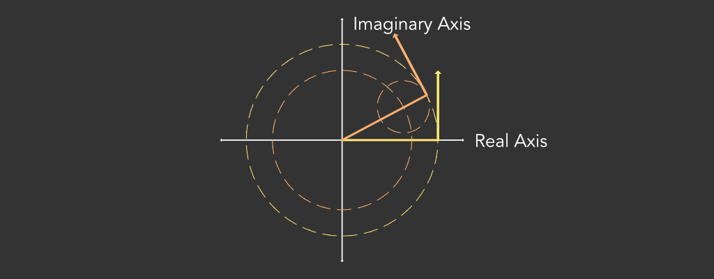
Before we dig into the math, we need to understand the key insight that led Joseph Fourier to his discovery. He found that any path through space can be expressed as a sum of circles that are rotating at different frequencies. The cover for this post illustrates this. If this kinda sounds like gibberish, that’s okay for now. But keep it in the back of your mind as we run through the math—all we are doing is attaching rotating circles to each other to trace a pattern through space. Now, the math. Let’s consider how we can achieve rotation in the complex plane using Euler’s formula.

visual showing Euler's formula

\[e^{i(\phi)} = \cos(\phi) + i \sin(\phi)\]

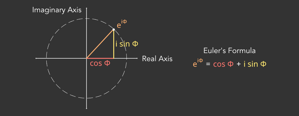
Remember that the complex plane has the real axis horizontally, and the complex axis vertically. Therefore, when we plug in some $\phi$ into the equation, we get a vertical component which is equal to the $\sin(\phi)$ and a horizontal component equal to the $\cos(\phi)$. This traces the unit circle in the complex plane as we increase $\phi$. Just take a second to think about how fascinating that is. Euler’s number, a constant for growth, when raised to an imaginary power, traces out a circle in the complex plane. Truly amazing.

There are a few different ways to arrive at this formula, and typically it is taught by plugging $i(\phi)$ into the Taylor polynomial for $e^x$. By performing a little bit of algebra, the resulting expression can be separated and factored to arrive at the taylor series for cosine, and the imaginary unit multiplied by the series for sine. But I’d like to take a look at a more intuitive explanation that—in my opinion—makes the equation even more beautiful.

Consider a ball on a string that is spinning horizontally. As the ball traces the circle, its velocity at a given point in time is along the tangential axis. At this same time, the force acting on the ball is on the radial axis. In other words, when the ball is moving, it is constantly being steered to its side. The result is that the ball doesn’t speed up or slow down. Instead, it changes direction continuously as it traces out a circle.

circular motion force diagram

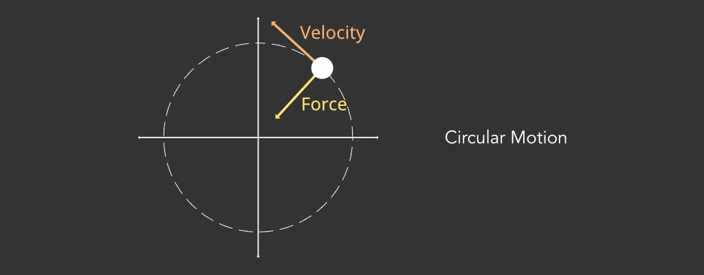
In the complex plane, we can obtain a perpendicular direction multiplying our velocity by i. Let’s write a differential equation for the velocity of a point in circular motion using this observation and solve it.

\[\begin{aligned} {dv \over dt} &= iv \\ \\ \int {dv \over v} &= \int {i dt} \\ \\ \ln v &= it + C_0 \\ \\ v &= C_1e^{kt} \end{aligned}\]

Bringing forth our prior knowledge that velocity is being steered in a circle gives us an interesting insight: Growth in a perpendicular direction is circular. This definition connects to the fact that euler’s number can be defined by continuously compounding interest. It’s not necessarily a rigorous way to arrive at Euler’s formula, but it certainly offers an intuition that the other methods of derivation do not.

Roots of Unity

The next important mathematical idea involves using Euler’s formula to solve a seemingly simple equation:

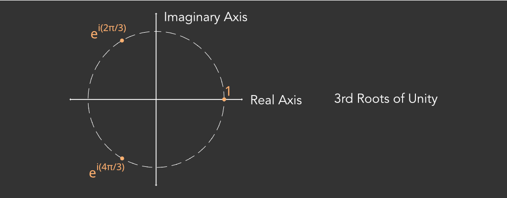
\[z^n = 1\]

The most obvious solution is $z=1$, but remember that by the fundamental theorem of algebra, this equation must have exactly $n$ complex roots. Also recall that multiplication of two complex numbers is the same as multiplying their magnitude and adding the angles between them and the real axis. Since our final magnitude is $1$ (and magnitudes are nonnegative real numbers), the magnitude of $z$ must also be one. Since all points in the complex plane with magnitude one are captured by Euler’s formula, let’s bring it in to solve our equation.

\[\begin{align}z^n &= 1 \\ \\ \text{let } z = e^{ix} \rightarrow e^{(ix)n} &= e^{i(2 \pi m)} \\ \\ nx &= 2 \pi m \\ \\ x &= {2 \pi \over n} m \\ \\ z = e^{ix} \rightarrow z &= e^{i {2 \pi \over n} m}\end{align}\]

Most of the algebra is relatively straightforward. The only slightly misleading tactic is where we substitute $e^{i(2\pi m)}$ for one, since any number of complete rotations will still get us to the same point. Otherwise, the formula simply states that the roots of unity are equally spaced on the unit circle in the complex plane. The roots of unity have many important properties relevant in various unexpected areas of math.

roots of unity

In the case of the discrete Fourier transform, the most important property is by far the sum of the roots. Let’s consider what happens as we take the total sum of our roots in the complex plane. The intuitive result is that the points are evenly spaced around a disc, and so their center of mass will be at the origin. We can more formally prove this later, but this intuition is essential for the discrete Fourier transform.

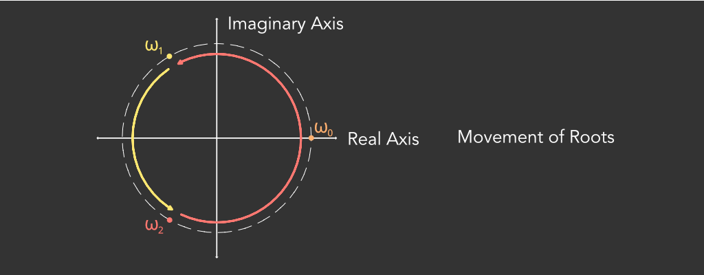
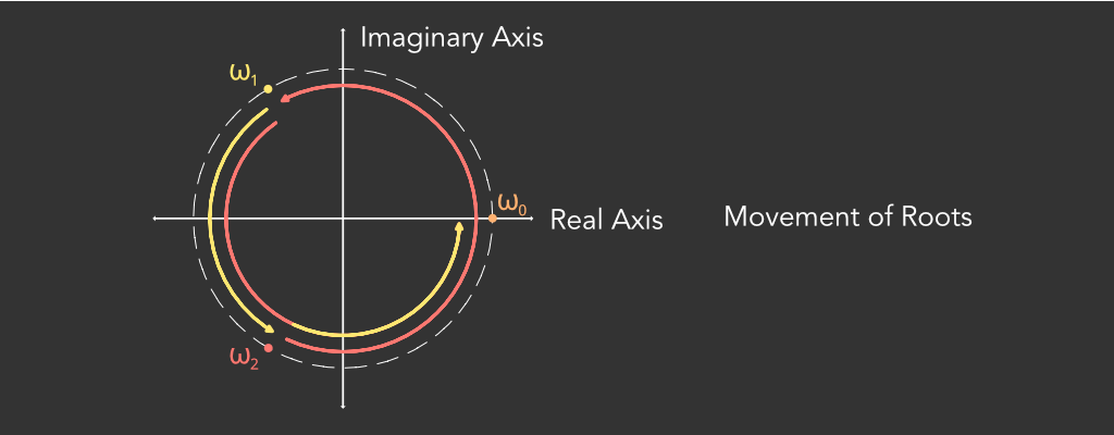
Bear with me for a minute. This next part is sort of a leap of faith. We are going to consider what happens as we raise the roots of unity to various powers. We’ll consider the $n$-th roots, meaning any of the roots raised to the n power will be one. Let’s label each of the $n$ roots as $\omega_0$ to $\omega_{n-1}$. If we increase the power of any of these roots, the new value will rotate by the initial rotation. In other words, we are going to move from $\omega_n$ to $\omega_{n+k}$. Notice how the bigger $k$ is, the faster that the root traces a circle.

movement of roots of unity

Here is the critical idea: We can use powers of roots of unity as different frequencies of rotation in the complex plane. We assign an amplitude to each frequency. To sample the value of our sum at a given time, we raise each root of unity to a power representing progress through time, multiply them by their frequency, and add them up. This may not seem like a grand idea, but it gives birth to the inverse discrete Fourier transform. The discrete Fourier transform samples each of these frequencies at whole number powers, and uses the same number of frequencies as samples. This is the formula:

\[x(n) = \sum_{k=0}^{N-1} X(k)e^{i{2\pi \over N}kn}\]

All that we do here is define a point in the time domain, $x(n)$, as the sum of the amplitudes, $X(k)$, multiplied by the root of unity for that frequency to the power of the sample point. Another thing to note is that instead of having a frequency of $N$, we shift to have a frequency of zero. Interestingly these are exactly the same at each sample point, and you can imagine that a circle with a frequency of $N$, will make a complete rotation at each sample, so that by the end of $N$ samples, it has made $N$ revolutions (This will come in handy later).

The Dirac Delta Function

We have an understanding of the inverse Fourier transform, but it doesn’t necessarily give any insight into how we can actually calculate the forward transform. To do this, we’re going to start with signals, and try to make some meaning as to their output. We can choose to build a signal with three frequencies. It doesn’t seem like too few or too many, but it doesn’t really matter how many we choose. With three frequencies, we will accordingly get three samples in the time domain.

To start off, we can give an amplitude of one to each of the frequencies, just to get our bearings. To calculate the time domain value at each sample, we trace the frequencies and add them together after each step. Each of our amplitudes is one, and we can visualize this by combining our roots of unity at each sample, and then moving them to the next position.

repeated movements of roots of unity

At the first step, we have all points at a zero degree angle, so their sum is three. We also know the second position, all of the roots are the third roots of unity, so their sum is zero. Now we must consider the third point in time. Let’s trace our roots as they move around. The frequency zero root stays put. The frequency one root moves to the second root of unity. The frequency two root moves to the fourth root, which is equal to the first root. The result is that at the final point in time, we have the original roots of unity, which sum to zero

We see an interesting pattern emerge. When all of the frequencies are one, the initial signal is equal to the number of frequencies, and the other samples are at a magnitude of zero. What is more interesting perhaps, is that this pattern continues when we add more frequencies. If all of their magnitudes are one, then the output is zero at all frequencies which aren’t zero. This isn’t necessarily an intuitive topic. I encourage you to trace out the various patterns for some set of roots of unity at different times. Sometimes they overlap, but except for the initial signal, the sum is zero. This is known as destructive interference.

Since we could really choose any set of roots of unity, it’s worth proving that the sum is always zero. Let’s consider the -th roots of unity raised to some power . Their sum can be expressed as the following:

\[S = \sum_{k=0}^{N-1} e^{i{2 \pi \over n}km}\]

When $m$ is zero, or a multiple of $n$, all roots are one, so the sum is equal to the number of roots that we add. For all other $m$, recognize that this is a geometric series with a common ratio equal to the first root of unity to the power of $m$. The initial term is one. At this point we can choose to derive the equation for the sum of a finite geometric series, or just take it as a given. Here we just use the given formula.

\[\begin{align} S &= { {a_1 (1-r^n)} \over {1-r} } \\ \\ &= { {1(1 - e^{i{2 \pi \over n} mn})} \over 1 - e^{i{2 \pi \over n} } } \\ \\ &= {1 - e^{i{2 \pi} (m)} \over 1 - e^{i{2 \pi \over n} } } \\ \\ &= {0 \over 1 - e^{i{2 \pi \over n} } } \\ \\ &= 0 \end{align}\]

In general, this pattern is called lol the delta function. The delta function has some unique properties in the continuous Fourier transform, but we can understand it simply to be equal to $N$ at the beginning of our signal, and zero at the rest of the samples. We can tactfully use this delta function to reverse engineer signals and break them down into their frequencies. This is the most powerful idea of the Fourier transform.

The Fourier Transform

Let’s try to manufacture a signal by cleverly choosing frequencies. A solid start is the dirac delta function, which we just derived. With four signals of amplitude of one, we get the values $[4, 0, 0, 0]$ in the time domain (Note that we use vector notation). Knowing that the inverse transform multiplies all frequencies by their respective amplitudes, we conclude that if we don’t change their relative magnitudes, we will have the same constructive and destructive interference.

Therefore, to construct a signal of $[1, 0, 0, 0]$ in the time domain, our signal in the frequency domain becomes $[¼, ¼, ¼, ¼]$. We can also generalize this logic. To construct a signal in the time domain $[a, 0, 0, 0]$, we spread the amplitude across all the frequencies to get frequencies $[a/N, a/N, a/N, a/N]$. This is a key insight:

The Fourier transform uses the dirac delta function to decompose any signal.

Let’s work through decomposing some signal $[a, b, c, d]$. The first thing to note is that we can combine two sets of signals to get a signal which is equal to the sum of their respective signals. This means that if we have one set of frequencies which gives $[a, 0, 0, 0]$ and another which yields $[0, b, 0, 0]$, then we can add them together to get a frequency domain that transforms to $[a, b, 0, 0]$. This can be derived from the formula for the inverse discrete transform or concluded intuitively. Two attached circles rotating with the same frequency can be described by one circle with radii that are the sum of the other two.

rotating circles described by their sum

Knowing that our signal can be expressed as the sum of different delta functions leaves us with only one problem to solve. We know how to construct a signal when the constructive interference occurs at the beginning of the period. How can we more carefully choose when this should occur? The answer is brilliant. Instead of scaling our amplitudes along only the real axis, we can scale them in the complex plane! This can be viewed as choosing a point on our circle to begin the rotation, instead of just how large the circle is. We accomplish this by using Euler’s formula.

To determine how far we should offset each amplitude, we realize that in each time step, a frequency n wave will move n roots of unity. Therefore, if we want to have constructive interference after the first timestep passes, we should offset each root backwards by the same number of roots as their frequency. To have it occur after the second step, we double this offset. In general, we offset each frequency by the time we want the occurrence multiplied by its frequency.

At this point, we have all of the tools to build the discrete Fourier transform. For each value in the time domain, we need to go over all of the frequencies, and find their contributions to the delta function which is zero at all other times and add them. And this works! However, in the actual discrete Fourier transform, we reverse the order. We go through each frequency and find their contribution to each time signal. Either is correct, but the latter lends itself better to being computed quickly (the fast Fourier transform). Regardless, here is the discrete Fourier transform.

\[X(k) = {1 \over N} \sum_{n=0}^{N-1} x(n)e^{-{2i \pi \over N}nk}\]

By this point, this formula should really feel somewhat natural. I’d like to point out a few different things though. We’ve chosen to divide the amplitude by the number of samples after the sum, but this is purely to save computations. We could just as well divide each term in the sum by the number of frequencies and get the same result. A second important thing to note is that the value of the time domain by no means has to be a real value. We can just as well choose a value in the complex plane, and all the frequencies will be rotated by the necessary amounts. The DFT is unreasonable in its robustness. It just requires a set of numbers somewhere in the complex plane, and can output the corresponding frequencies.

Putting It Together

With an understanding of the Fourier transform, let’s build a little project to test our understanding. What I want to do is allow the user to input a set of points on the screen with the mouse. We’ll let the points represent the complex plane. From there, we can run the discrete Fourier transform to convert from our points into our frequencies. If we iterate over each frequency, we add its contribution to the total signal by creating a circle with a radius equal to its magnitude. Note that we can evaluate our DFT with more resolution by just plugging in noninteger sample points. Think through why this is true.

This seems to work, and does hit all of our points, but we notice some weird behavior. Instead of getting a star with relatively straight lines, the DFT seems to oscillate very quickly between points. This behavior is due to the high frequency waves. Let’s recall from earlier how the DFT is periodic. The same way a frequency $N$ wave is equal to a frequency $0$ wave at all sample points. A frequency $N-1$ wave is equal to a frequency $-1$ wave, which we can imagine to rotate backwards slowly.

We could alter our DFT algorithm, but we can actually just write code to more cleverly sample our DFT. Whenever we add a new frequency, we decide if it is greater than half of the max, and if it is, we draw it as going the opposite direction by subtracting $N$ from the frequency. One more change we can make is the order of draw frequencies. We can sort frequencies by magnitude, or just go from lowest to highest. I’m going to keep it simple and draw the lowest frequencies first. Let’s take a look at how this looks.

There we go! You can view the source code for this demo here. There’s still a lot we could do with this, but let’s save it for later. Here are a few different ideas that would take the Fourier transform to the next level:

We could implement the fast Fourier transform to reduce the computation time.
We could extend the Fourier transform into higher dimensions to compress data such as images (similar to how JPEG works).
We could capitalize on the properties of the Fourier transform to implement image filters.
We could create a noise filter for a microphone to remove background noise.

At this point, I’m happy with our progress, but I’ll consider coming back to some of these ideas in the future. The project that originally pointed me to the Fourier transform was our fluid simulation project, as the ocean surface itself can be expressed by its spectrum, which oceanographers have worked to measure. I plan to continue that project in the next post, but I wanted to step out of the context of that project to dive into the Fourier transform for this post. Thanks for reading!

References

This was by far the hardest I’ve pushed myself to learn a topic. I couldn’t have done it without reading many papers, articles, and posts. Here are the sites that I referred to when writing and developing this post: